Viscous Flow in the Mantle

Viscous Flow in the Earth's Mantle

In our recent papers Conrad, Behn, & Silver [2007] and Conrad & Behn [2010] (see citations below) we computed mantle flow driven by the combination of three components:

(1) mantle density heterogeneities inferred from the S20RTSb seismic tomography model of Ritsema et al. [2004]
(2) NUVEL-1A plate motions [DeMets et al., 1994] in the no-net-rotation reference frame
(3) net lithosphere lithosphere rotation, as inferred from the HS3 (Pacific hotspot) model [Gripp & Gordon, 2002].

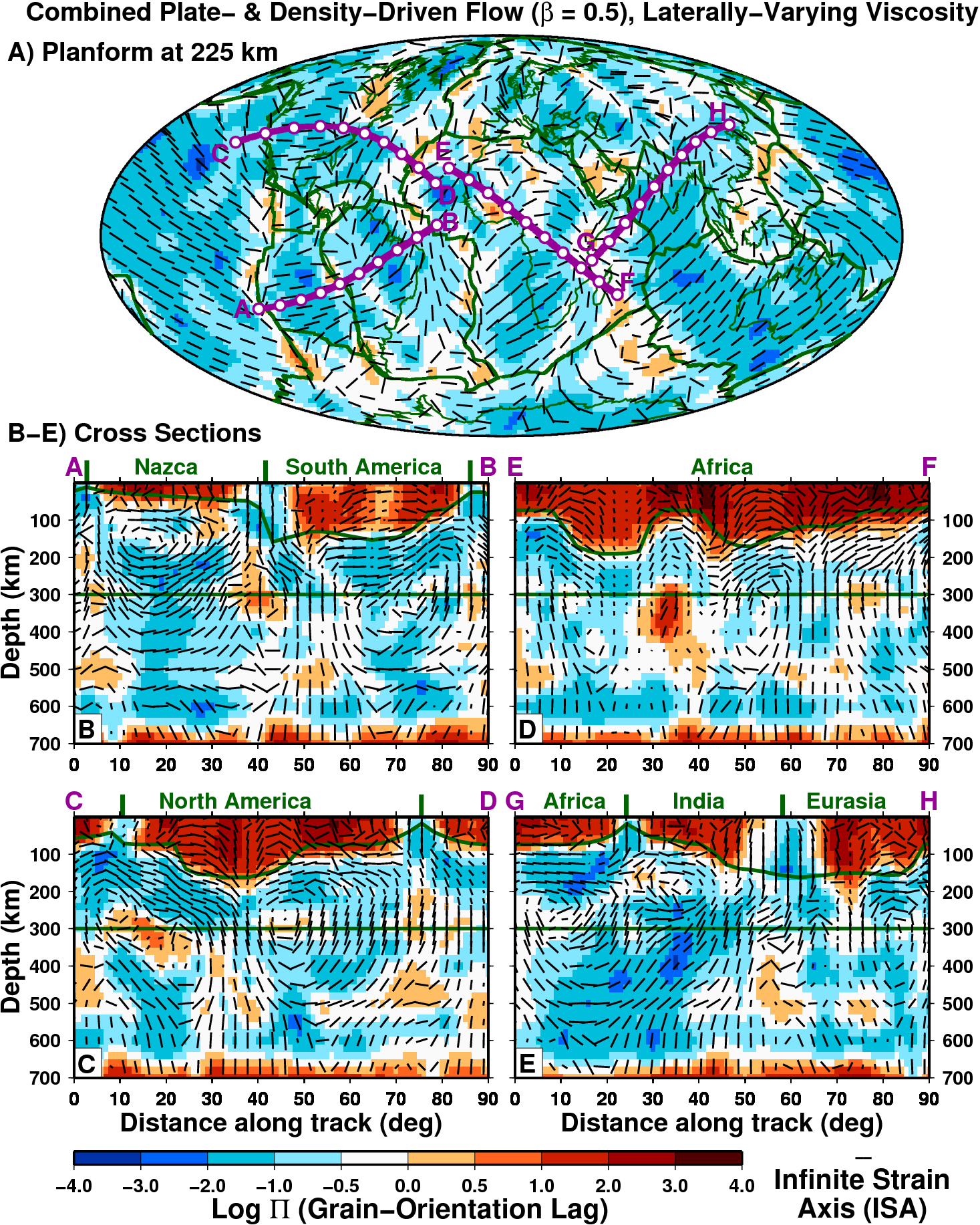
We then used observations of seismic anisotropy to constrain the best combination of these three (density-driven, plate-driven, and net-rotation-driven) flow fields. The result is a global model of viscous mantle flow (shown in the above figure). Here, we provide downloadable files of the flow field itself, as well as the infinite strain axis (ISA) and PI parameter (both defined by Kaminski & Ribe [2002]), which can be used to infer anisotropic fabric.

Updates

May 2010: Our mantle flow model has been updated based on the recent publication of Conrad & Behn [2010] in Gcubed (see citation below). The files below are now from the model presented in the 2010 Gcubed paper, and assume beta=0.5 and alpha=0.2. If you would like the files associated with the 2007 JGR paper, then they can be accessed here, on an older version of this page.

January 2008: We have improved our method for estimating the ISA and PI parameters (by improving the precision of our code). The improved results provide a smoother ISA field, and thus slighly lower values of PI throughout the asthenosphere. Therefore, we have replotted some of the key figures from the Conrad, Behn, and Silver [JGR, 2007] paper:
Figure 4
Figure 5
Figure S1
Figure S2
Updated Supplementary README Text (for figures S1 and S2)

Global Mantle Flow Model for Download

The files below provide the global mantle flow model that is described in the Conrad & Behn [2010] Gcubed paper. Included are the temperature, viscosity, velocity, and stress fields for the entire mantle at two time steps: Time step 0 is for the present day, and time step 10 is for a time about 3.5 Million years from now. These files allow us to determine the present-day flow field and how it is currently changing with time (its first time-derivative). Also given are the anisotropic parameters ISA and PI, which were computed using the "calcpi" code (see below) as described by Conrad et al. [2007]. The details of how the flow field was calculated are described in the Conrad & Behn [Gcubed, 2010] paper, which you should cite if you use these files (see citation below).

Location/Temperature/Viscosity:
s20rtsb.inexhs3v.comb.0.xyzt.gz Time Step 0 (Gzipped Ascii File, 7.1 MB)
s20rtsb.inexhs3v.comb.10.xyzt.gz Time Step 10 (Gzipped Ascii File, 8.2 MB)
Format (5 columns):
1. (colatitude (radians measured from the north pole)
2. longitude (radians)
3. radius (measured as fraction of the earth's radius: CMB=0.55, 1.0=Surface)
4. temperature (relative measure between 1 at the CMB and 0 at the surface)
5. viscosity (multiply by 0.5e21 Pa s to make dimensional)

Flow Velocities:
s20rtsb.inexhs3v.comb.0.v.gz Time Step 0 (Gzipped Ascii File, 10.1 MB)
s20rtsb.inexhs3v.comb.10.v.gz Time Step 10 (Gzipped Ascii File, 10.1 MB)
Format (3 columns, dimensionless units - divide by 2018.9 to convert to cm/yr):
1. Theta (Positive Southward) Velocity
2. Phi (Positive Eastward) Velocity
3. Radial (Positive Upward) Velocity

Stress Field:
s20rtsb.inexhs3v.comb.0.str.gz Time Step 0 (Gzipped Ascii File, 20.6 MB)
s20rtsb.inexhs3v.comb.10.str.gz Time Step 10 (Gzipped Ascii File, 20.6 MB)
Format (6 columns, dimensionless units - multiply by 12.322 to convert to Pa):
1. Sigma_radial_radial
2. Sigma_radial_phi
3. Sigma_radial_theta
4. Sigma_phi_phi
5. Sigma_theta_phi
6. Sigma_theta_theta

Time Dependence: s20rtsb.inexhs3v.time.gz Time Step File (Gzipped Ascii File, <1 KB)
Format (5 columns)
1. Step Number
2. Total Elapsed Time (dimensionless units - multiply by 1.286E06 to convert to Myr)
3. Time for Step (dimensionless units - multiply by 1.286E06 to convert to Myr)
4. Total Elapsed Wall Clock Time (s)
5. Wall Clock Time for step (s)

Infinite Strain Axis: [s20rtsb.inexhs3v.comb.10.ehat.gz] (Gzipped Ascii File, 7.2 MB)
Format (3 columns):
1. Theta (Southward) Component
2. Phi (Eastward) Component
3. Radial (Upward) Component

PI Parameter: [s20rtsb.inexhs3v.comb.10.pi.gz] (Gzipped Ascii File, 3.2 MB)
Format (1 column):
1. PI value (dimensionless)

Plate-Driven Flow Field: [s20rtsb.exv.comb.0.xyzt.gz] [s20rtsb.exv.comb.0.v.gz] [s20rtsb.exv.comb.0.str.gz] [s20rtsb.exv.comb.10.ehat.gz] [s20rtsb.exv.comb.10.pi.gz]

Density-Driven Flow Field: [s20rtsb.inv.comb.0.xyzt.gz] [s20rtsb.inv.comb.0.v.gz] [s20rtsb.inv.comb.0.str.gz] [s20rtsb.inv.comb.10.ehat.gz] [s20rtsb.inv.comb.10.pi.gz]

Prediction of Anisotropic Crystal Fabric

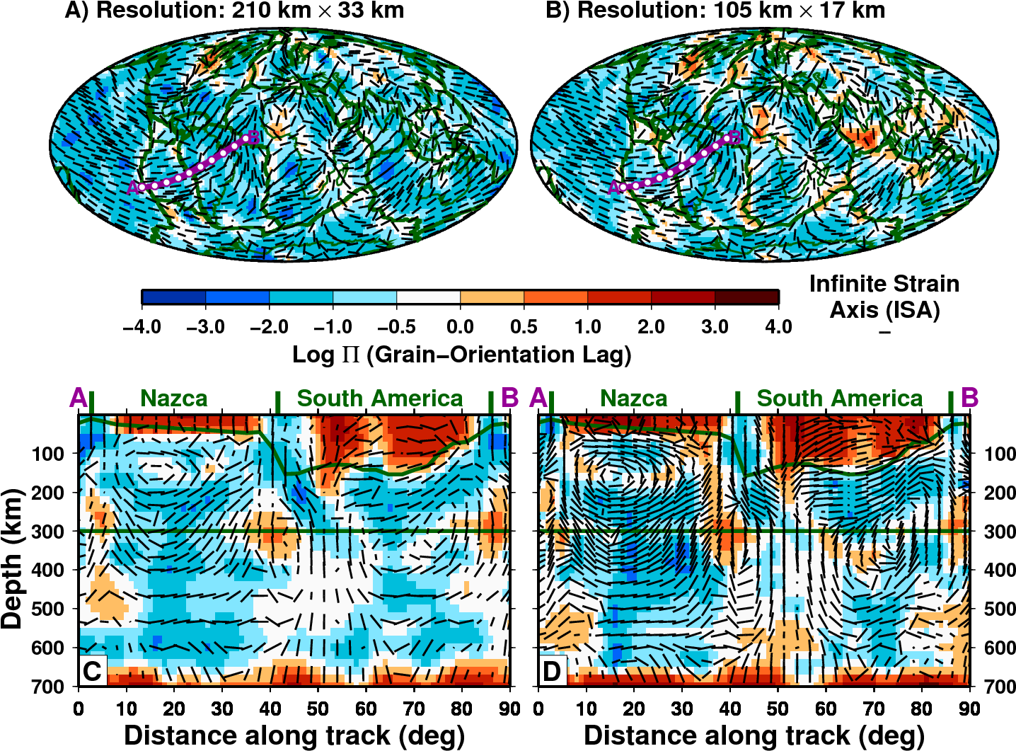
The strain deformations caused by mantle flow will deform olivine aggregates into a lattice-preferred orientation (LPO), generating a seismically anisotropic fabric. We use the above flow field to predict LPO for the asthenosphere by implementing Kaminski & Ribe's [2002] scheme for estimating crystal fabric from a given flow field. This method uses the infinite strain axis (ISA, the orientation of the long axis of the finite strain ellipsoid after an infinite amount of uniform strain) to approximate the LPO. Because the ISA can be estimated from an instantaneous flow field, time-dependent strain-accumulation is not necessary. However, if the flow field varies too rapidly in space or in time, then the ISA~LPO approximation is not valid. To determine where this approximation is valid, Kaminski & Ribe [2002] introduced the PI parameter that compares the rate of ISA developement with the rate of ISA rotation in the flow field. Where PI > 0.5, then the flow field rotates olivine crystals away from the ISA faster than the ISA can develop. In this case, the ISA is a poor approximation of LPO. Thus, it is important to make sure that PI < 0.5 before comparing predictions of ISA with observations. Fortunately, we have found that PI < 0.5 throughout most of the asthenosphere in most cases.

Our code for calculating PI and ISA from the above flow field is here:

calcpi fortran code: [calcpicode.tar.gz] (gzipped, tarred, directory, 10.6 KB)

Please cite Conrad, Behn, and Silver, [JGR, 2007] if you use the above code (see citation below).

Citations

Please cite the following paper if you use the calcpi code (see above) to predict anisotropic fabric:

Conrad, C.P., M.D. Behn, and P.G. Silver, Global mantle flow and the development of seismic anisotropy: Differences between the oceanic and continental upper mantle, Journal of Geophysical Research, 112, B07317, doi:10.1029/2006JB004608, 2007. [online version] [reprint] [auxiliary material]

Please cite the following paper if you use the mantle flow model or the anisotropic predictions that were made form it:

Conrad, C.P., and M.D. Behn, Constraints on lithosphere net rotation and asthenospheric viscosity from global mantle flow models and seismic anisotropy, Geochemistry, Geophysics, Geosystems, 11, Q05W05, doi:10.1029/2009GC002970, 2010. [online version] [reprint] [theme issue]